pgamma(4,3,1)[1] 0.7618967Please note that there is a file on Canvas called Getting started with R which may be of some use. This provides details of setting up R and Rstudio on your own computer as well as providing an overview of inputting and importing various data files into R. This should mainly serve as a reminder.
Recall that we can clear the environment using rm(list=ls()) It is advisable to do this before attempting new questions if confusion may arise with variable names etc.
Let \(X\sim Gamma(3,1)\). Find \(P(X\leq 4)\) and \(P(X>2)\).
Further, let \(Y\sim Gamma(2,0.5)\). Find \(P(Y<1)\) and the value of the pdf at \(y=3\). Create a plot of \(Y\sim Gamma(2,0.5)\).
Hint: Adapt the R code met previously for other distributions. In particular, the help("pgamma") R code should be useful in determining the arguments/options.
help("pgamma")pgamma(4,3,1)[1] 0.76189671-pgamma(2,3,1)[1] 0.6766764Or
pgamma(2,3,1,lower.tail=F)[1] 0.6766764\(P(Y<1):\)
pgamma(1,2,0.5)[1] 0.09020401and the value of the pdf at y=3:
dgamma(3,2,0.5)[1] 0.1673476We first create a sequence of numbers (inputs) between 0 and 20 and then find the corresponding values of the distribution function. Finally we plot these against each other.
y<-seq(0,20, length=10000)
dy<-dgamma(y,2,0.5)
plot(y,dy, xlab="y value",type="l", ylab="Density", main="Gamma(2,0.5) Distribution")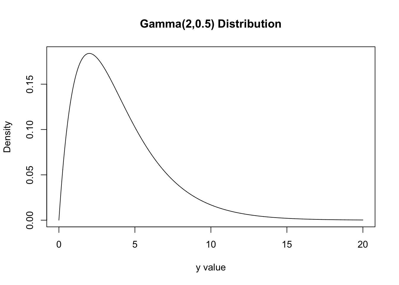
In this example we will perform a gamma regression on an in-built dataset in R (wafer) using the log link function. The outcome is measuring resistance of a wafer in a physics experiment. The predictor/independent variables are \(x_1,\ldots,x_3\).
install.packages("faraway")library(faraway)
data(wafer)
plot(density(wafer$resist))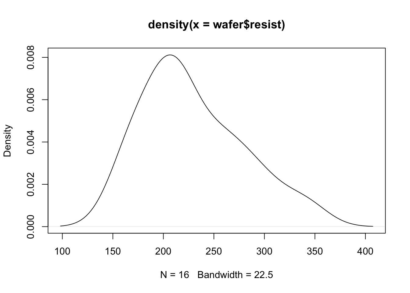
help("ks.test")
library(MASS)
help("fitdistr")
fitdistr(wafer$resist, "gamma")
shape rate
23.09377758 0.10072802
( 8.09441180) ( 0.03568919)ks.test(wafer$resist, pgamma, shape=23.1, rate=0.1)
    Exact one-sample Kolmogorov-Smirnov test

data:  wafer$resist
D = 0.16066, p-value = 0.7458
alternative hypothesis: two-sidedGammaReg <- glm(formula = resist ~ x1 + x2 + x3,
family = Gamma(link = "log"),
data = wafer)
summary(GammaReg)
Call:
glm(formula = resist ~ x1 + x2 + x3, family = Gamma(link = "log"),
    data = wafer)

Coefficients:
            Estimate Std. Error t value Pr(>|t|)
(Intercept)  5.41553    0.05305 102.083  < 2e-16 ***
x1+          0.12110    0.05305   2.283 0.041474 *
x2+         -0.29981    0.05305  -5.651 0.000107 ***
x3+          0.18240    0.05305   3.438 0.004909 **
---
Signif. codes:  0 '***' 0.001 '**' 0.01 '*' 0.05 '.' 0.1 ' ' 1

(Dispersion parameter for Gamma family taken to be 0.01125723)

    Null deviance: 0.69784  on 15  degrees of freedom
Residual deviance: 0.13741  on 12  degrees of freedom
AIC: 152.53

Number of Fisher Scoring iterations: 4
The output above shows the significance of the predictor variables and the coefficients
Finally, we evaluate the model using Deviance
anova(GammaReg, test="Chisq")Analysis of Deviance Table
Model: Gamma, link: log
Response: resist
Terms added sequentially (first to last)
Df Deviance Resid. Df Resid. Dev Pr(>Chi)
NULL 15 0.69784
x1 1 0.05059 14 0.64725 0.0340206 *
x2 1 0.37740 13 0.26985 7.034e-09 ***
x3 1 0.13244 12 0.13741 0.0006035 ***
---
Signif. codes: 0 '***' 0.001 '**' 0.01 '*' 0.05 '.' 0.1 ' ' 1