dbinom(2,10,0.4)[1] 0.1209324Please note that there is a file on Canvas called Getting started with R which may be of some use. This provides details of setting up R and Rstudio on your own computer as well as providing an overview of inputting and importing various data files into R. This should mainly serve as a reminder.
Recall that we can clear the environment using rm(list=ls()) It is advisable to do this before attempting new questions if confusion may arise with variable names etc.
Let \(X\sim Bin(10,0.4)\). Calculate the following. The help("pbinom") function may be of use.
Find \(P(X=2)\).
Now we use the distribution function pbinom to find \(P(X<5)\).
Generate 30 random values from \(Bin(20,0.1)\).
Plot the Probability Mass Function (PMF) of \(Bin(15,0.3)\). Hint: create a sequence of numbers (inputs) between 1 and 15 and then find the corresponding values of the distribution function (PMF in this case). Finally, we plot these against each other.
dbinom(2,10,0.4)[1] 0.1209324pbinom(4,10,0.4)[1] 0.6331033rbinom(30,20,0.1) [1] 0 0 3 0 2 1 4 4 0 3 3 4 3 2 2 4 1 3 3 3 2 3 1 2 2 4 2 0 3 1?plotx<-seq(1,15, length=15)
dx<-dbinom(x,15,0.3)
plot(x,dx, xlab="x value",type="p", ylab="Probability", main="Binom(15,0.3) Distribution")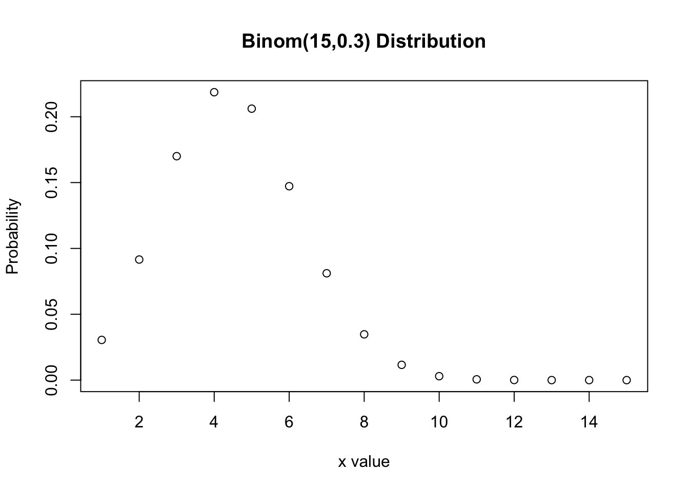
In this example we will use the logistic regression procedure on the Logistic Regression (Quality) dataset. This dataset has a number of variables related to the quality of care. We firstly assume that we have independence of observations. Further remarks about assumptions will be made in the steps below. Please follow the steps below.
The first model we will consider is where PoorCare is the dependent variable and AcuteDrugGapSmall is the independent variable. Note that PoorCare is a binary variable, satisfying an assumption of the procedure. Inspection of AcuteDrugGapSmall indicates the variable can be treated as continuous; therefore a further assumption is satisfied. We do not need to consider multicollinearity in this case as we only have one independent variable. The final assumption is linearity in the sense that Logit(PoorCare) and AcuteDrugGapSmall should be linearly related - we assume that this is true in this case.
We firstly import and check the data:
library(foreign)
Quality<-read.spss(file.choose(), to.data.frame = T)head(Quality) MemberID InpatientDays ERVisits OfficeVisits Narcotics DaysSinceLastERVisit
1 1 0 0 18 1 731
2 2 1 1 6 1 411
3 3 0 0 5 3 731
4 4 0 1 19 0 158
5 5 8 2 19 3 449
6 6 2 0 9 2 731
Pain TotalVisits ProviderCount MedicalClaims ClaimLines StartedOnCombination
1 10 18 21 93 222 0
2 0 8 27 19 115 0
3 10 5 16 27 148 0
4 34 20 14 59 242 0
5 10 29 24 51 204 0
6 6 11 40 53 156 0
AcuteDrugGapSmall PoorCare
1 0 0
2 1 0
3 5 0
4 0 0
5 0 0
6 4 1QualityLogit<-glm(PoorCare~AcuteDrugGapSmall, data=Quality, family="binomial")
summary(QualityLogit)
Call:
glm(formula = PoorCare ~ AcuteDrugGapSmall, family = "binomial",
    data = Quality)

Coefficients:
                  Estimate Std. Error z value Pr(>|z|)
(Intercept)       -1.79086    0.28220  -6.346 2.21e-10 ***
AcuteDrugGapSmall  0.25762    0.06451   3.994 6.50e-05 ***
---
Signif. codes:  0 '***' 0.001 '**' 0.01 '*' 0.05 '.' 0.1 ' ' 1

(Dispersion parameter for binomial family taken to be 1)

    Null deviance: 147.88  on 130  degrees of freedom
Residual deviance: 124.54  on 129  degrees of freedom
AIC: 128.54

Number of Fisher Scoring iterations: 5anova(QualityLogit, test="Chisq")Analysis of Deviance Table
Model: binomial, link: logit
Response: PoorCare
Terms added sequentially (first to last)
Df Deviance Resid. Df Resid. Dev Pr(>Chi)
NULL 130 147.88
AcuteDrugGapSmall 1 23.336 129 124.54 1.36e-06 ***
---
Signif. codes: 0 '***' 0.001 '**' 0.01 '*' 0.05 '.' 0.1 ' ' 1install.packages("lmtest")library(lmtest)
waldtest(QualityLogit, test="Chisq")Wald test
Model 1: PoorCare ~ AcuteDrugGapSmall
Model 2: PoorCare ~ 1
Res.Df Df Chisq Pr(>Chisq)
1 129
2 130 -1 15.95 6.504e-05 ***
---
Signif. codes: 0 '***' 0.001 '**' 0.01 '*' 0.05 '.' 0.1 ' ' 1From this table we see that the Wald test shows that the coefficient of AcuteDrugSmallGap, i.e. \(\beta_1\) is significantly different to 0. The Deviance statistic is also significant. Using the theory in the lecture notes we conclude that the model is: \[ logit(\hat{p})=-1.791+0.258x_1 \quad \text{or}\quad \hat{p}=\frac{e^{-1.791+0.258x_1}}{1+e^{-1.791+0.258x_1}}, \] where \(x_1\) denotes AcuteDrugGapSmall and \(\hat{p}\) is the estimated probability of receiving poor care. Note that the Fisher scoring iterations indicate how quickly the MLEs for the coefficients in the model converge.
The following code provides \(e^\beta\) along with a confidence interval for the coefficient, which helps our analysis
exp(cbind(OR = coef(QualityLogit), confint(QualityLogit))) OR 2.5 % 97.5 %
(Intercept) 0.1668162 0.09262101 0.2818085
AcuteDrugGapSmall 1.2938500 1.15026698 1.4848021Note that \(e^\beta=1.294\), indicating that increasing the independent variable, AcuteDrugsSmallGap, by 1 unit will increase the odds of PoorCare by 29.4%. The 95% confidence interval for \(e^\beta\) is \((1.15,1.484)\) - it is good that the confidence interval does not include 1, otherwise this would represent no change to the odds of the outcome.
We next use the DescTools package to calculate some pseudo\(R^2\) statistics.
install.packages("DescTools")library(DescTools)
PseudoR2(QualityLogit, which=c("CoxSnell", "Nagelkerke")) CoxSnell Nagelkerke
0.1631750 0.2411715 We see that Nagelkerke’s \(R^2\) indicates that 24.1% of the variation in the outcome is accounted for by the model (Cox and Snell: 16.3%)
Finally, we further evaluate the model using the Hosmer and Lemeshow test:
install.packages("generalhoslem")library(generalhoslem)
logitgof(Quality$PoorCare, fitted(QualityLogit))
    Hosmer and Lemeshow test (binary model)

data:  Quality$PoorCare, fitted(QualityLogit)
X-squared = 1.9916, df = 3, p-value = 0.5741
The Hosmer and Lemeshow test shows that we have a good model fit (not significant).
We now include another independent variable, StartedOnCombination. As the new variable is categorical, we must inform R using the following code:
Combination<-factor(Quality$StartedOnCombination)QualityLogit2<-glm(PoorCare~AcuteDrugGapSmall+Combination, data=Quality, family="binomial")
summary(QualityLogit2)
Call:
glm(formula = PoorCare ~ AcuteDrugGapSmall + Combination, family = "binomial",
    data = Quality)

Coefficients:
                  Estimate Std. Error z value Pr(>|z|)
(Intercept)       -2.07335    0.31625  -6.556 5.52e-11 ***
AcuteDrugGapSmall  0.28600    0.06911   4.138 3.50e-05 ***
Combination1       3.43061    1.15381   2.973  0.00295 **
---
Signif. codes:  0 '***' 0.001 '**' 0.01 '*' 0.05 '.' 0.1 ' ' 1

(Dispersion parameter for binomial family taken to be 1)

    Null deviance: 147.88  on 130  degrees of freedom
Residual deviance: 112.25  on 128  degrees of freedom
AIC: 118.25

Number of Fisher Scoring iterations: 5
Note that the Fisher scoring iterations indicate how quickly the MLEs for the coefficients in the model converge.
Again we begin to evaluate the model using:
anova(QualityLogit2, test="Chisq")Analysis of Deviance Table
Model: binomial, link: logit
Response: PoorCare
Terms added sequentially (first to last)
Df Deviance Resid. Df Resid. Dev Pr(>Chi)
NULL 130 147.88
AcuteDrugGapSmall 1 23.336 129 124.54 1.36e-06 ***
Combination 1 12.293 128 112.25 0.0004545 ***
---
Signif. codes: 0 '***' 0.001 '**' 0.01 '*' 0.05 '.' 0.1 ' ' 1library(lmtest)
waldtest(QualityLogit2, test="Chisq")Wald test
Model 1: PoorCare ~ AcuteDrugGapSmall + Combination
Model 2: PoorCare ~ 1
Res.Df Df Chisq Pr(>Chisq)
1 128
2 130 -2 22.791 1.125e-05 ***
---
Signif. codes: 0 '***' 0.001 '**' 0.01 '*' 0.05 '.' 0.1 ' ' 1We see that the Wald test shows that the coefficients of both independent variables i.e. \(\beta_1\) and \(\beta_2\) are significantly different to 0. The Deviance statistic is also significant.
We conclude that including the variable AcuteDrugGapSmall in logistic regression significantly improves the model and also that including both AcuteDrugGapSmall and StartedOnCombination significantly improves the model even further. Therefore, the model in this case is: \[ logit(\hat{p})=-2.073+0.286x_1+3.431x_2 \quad \text{or}\quad \hat{p}=\frac{e^{-2.073+0.286x_1+3.431x_2 }}{1+e^{-2.073+0.286x_1+3.431x_2 }}, \] where \(x_1\) denotes AcuteDrugGapSmall, \(x_2\) denotes StartedOnCombination and \(\hat{p}\) is the estimated probability of receiving poor care.
As we will now have two independent variables we must check for no multicollinearity using the following R code:
install.packages("car")library(car)
vif(QualityLogit2)AcuteDrugGapSmall Combination
1.022965 1.022965 We see from the above table that both the VIF terms are around 1, satisfying the no-multicollinearity assumption - we require the VIF factors to be around 1, or at least \(0.01<VIF<5\).
The following code provides \(e^\beta\) along with a confidence interval for the coefficient, which helps our analysis
exp(cbind(OR = coef(QualityLogit2), confint(QualityLogit2))) OR 2.5 % 97.5 %
(Intercept) 0.1257643 0.06450324 0.2248477
AcuteDrugGapSmall 1.3310961 1.17478068 1.5444554
Combination1 30.8956101 4.27766048 629.2075641Neither confidence interval our predictor variables for \(e^\beta\) includes 1.
We next use the DescTools package to calculate some pseudo\(R^2\) statistics.
PseudoR2(QualityLogit2, which=c("CoxSnell", "Nagelkerke")) CoxSnell Nagelkerke
0.2381334 0.3519595 We see that Nagelkerke’s \(R^2\) indicates that 35.2% of the variation in the outcome is accounted for by the model (Cox and Snell: 23.8%)
Finally, we further evaluate the model using the Hosmer and Lemeshow test:
logitgof(Quality$PoorCare, fitted(QualityLogit2))
    Hosmer and Lemeshow test (binary model)

data:  Quality$PoorCare, fitted(QualityLogit2)
X-squared = 0.70579, df = 4, p-value = 0.9506Investigate the Penalty dataset to determine whether a logistic regression model may be used to predict the variable Scored from the three variables PSWQ, Anxious and Previous.
library(foreign)
Penalty2<-read.spss(file.choose(), to.data.frame = T)library(foreign)
Penalty2<-read.spss("Penalty2.sav", to.data.frame = T)PenaltyLogit<-glm(Scored~PSWQ+Anxious+Previous, data=Penalty2, family="binomial")
summary(PenaltyLogit)
Call:
glm(formula = Scored ~ PSWQ + Anxious + Previous, family = "binomial",
    data = Penalty2)

Coefficients:
             Estimate Std. Error z value Pr(>|z|)
(Intercept) -11.49256   11.80175  -0.974  0.33016
PSWQ         -0.25137    0.08401  -2.992  0.00277 **
Anxious       0.27585    0.25259   1.092  0.27480
Previous      0.20261    0.12932   1.567  0.11719
---
Signif. codes:  0 '***' 0.001 '**' 0.01 '*' 0.05 '.' 0.1 ' ' 1

(Dispersion parameter for binomial family taken to be 1)

    Null deviance: 103.638  on 74  degrees of freedom
Residual deviance:  47.416  on 71  degrees of freedom
AIC: 55.416

Number of Fisher Scoring iterations: 6probabilities2 <- predict(PenaltyLogit, type = "response")
logit2<-log(probabilities2/(1-probabilities2))par(mfrow=c(1,3))
plot(Penalty2$PSWQ,logit2, main = "Scatterplot of Logit vs PSWQ ",
xlab = "PSWQ", ylab = "logit(p)", frame = FALSE)
plot(Penalty2$Anxious,logit2, main = "Scatterplot of Logit vs Anxious ",
xlab = "Anxious", ylab = "logit(p)", frame = FALSE)
plot(Penalty2$Previous,logit2, main = "Scatterplot of Logit vs Previous ",
xlab = "Previous", ylab = "logit(p)", frame = FALSE)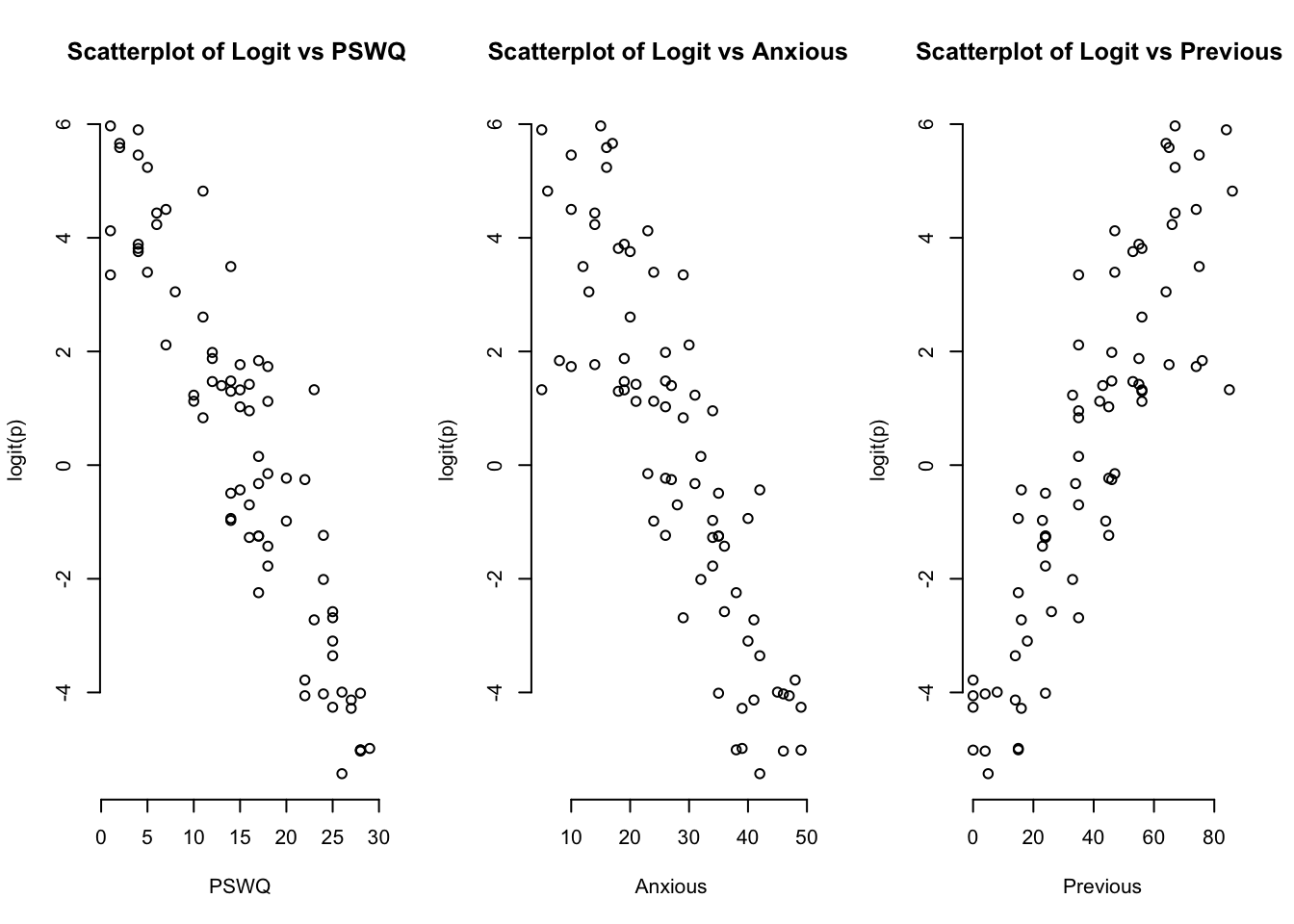
We can see by inspection that we have linearity in the sense of this procedure.
Now we check the no multicollinearity assumption
library(car)
vif(PenaltyLogit)
PSWQ Anxious Previous
1.089767 35.581976 35.227113