help("dpois")
dpois(3,0.75)
[1] 0.03321327ppois(2,0.75)[1] 0.9594946Please note that there is a file on Canvas called Getting started with R which may be of some use. This provides details of setting up R and Rstudio on your own computer as well as providing an overview of inputting and importing various data files into R. This should mainly serve as a reminder.
Recall that we can clear the environment using rm(list=ls()) It is advisable to do this before attempting new questions if confusion may arise with variable names etc.
In this example we let \(X\sim \text{Po}(0.75)\) and we calculate \(P(X=3)\) and \(P(X\leq 2)\), and we will plot this distribution.
help("dpois")
dpois(3,0.75)[1] 0.03321327ppois(2,0.75)[1] 0.9594946x<-seq(0,14, length=15)
dx<-dpois(x,0.75)
plot(x,dx, xlab="x value",type="p", ylab="Probability", main="Poisson(0.75) Distribution")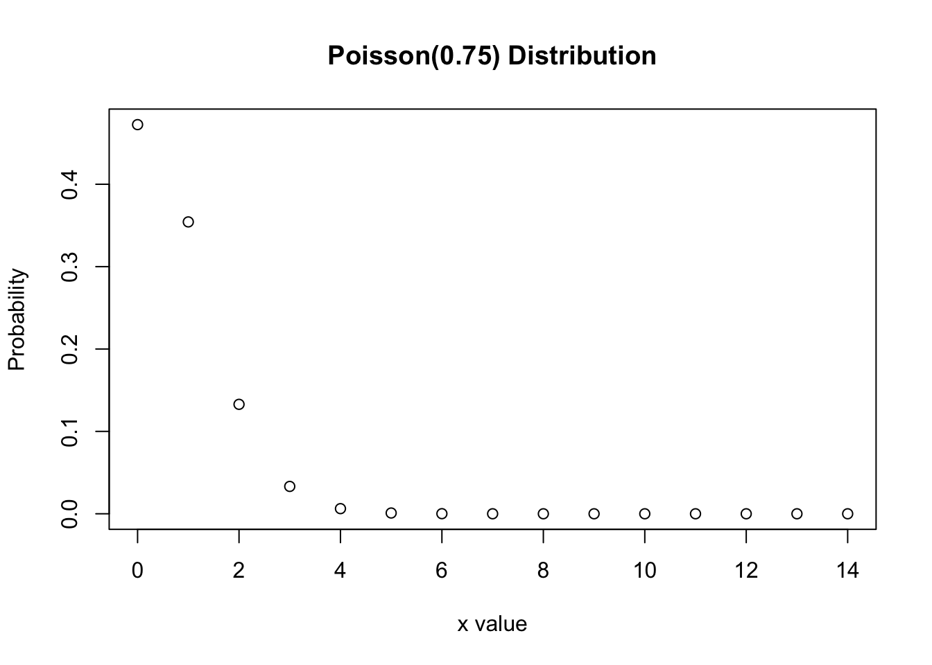
For \(Y\sim Po(1.5)\) find \(P(Y=1)\) and \(P(Y>3)\).
In this example we will create Poisson random numbers and then test to see whether the numbers generated follow a Poisson distribution.
Note: Everyone’s results will likely be different as this is a random process.
help("rpois")
RandomSample<-rpois(20,2.5)
RandomSample
[1] 1 1 3 1 1 4 2 1 2 2 4 2 3 1 2 2 1 3 1 3mean(RandomSample)[1] 2var(RandomSample)[1] 1.052632hist(RandomSample)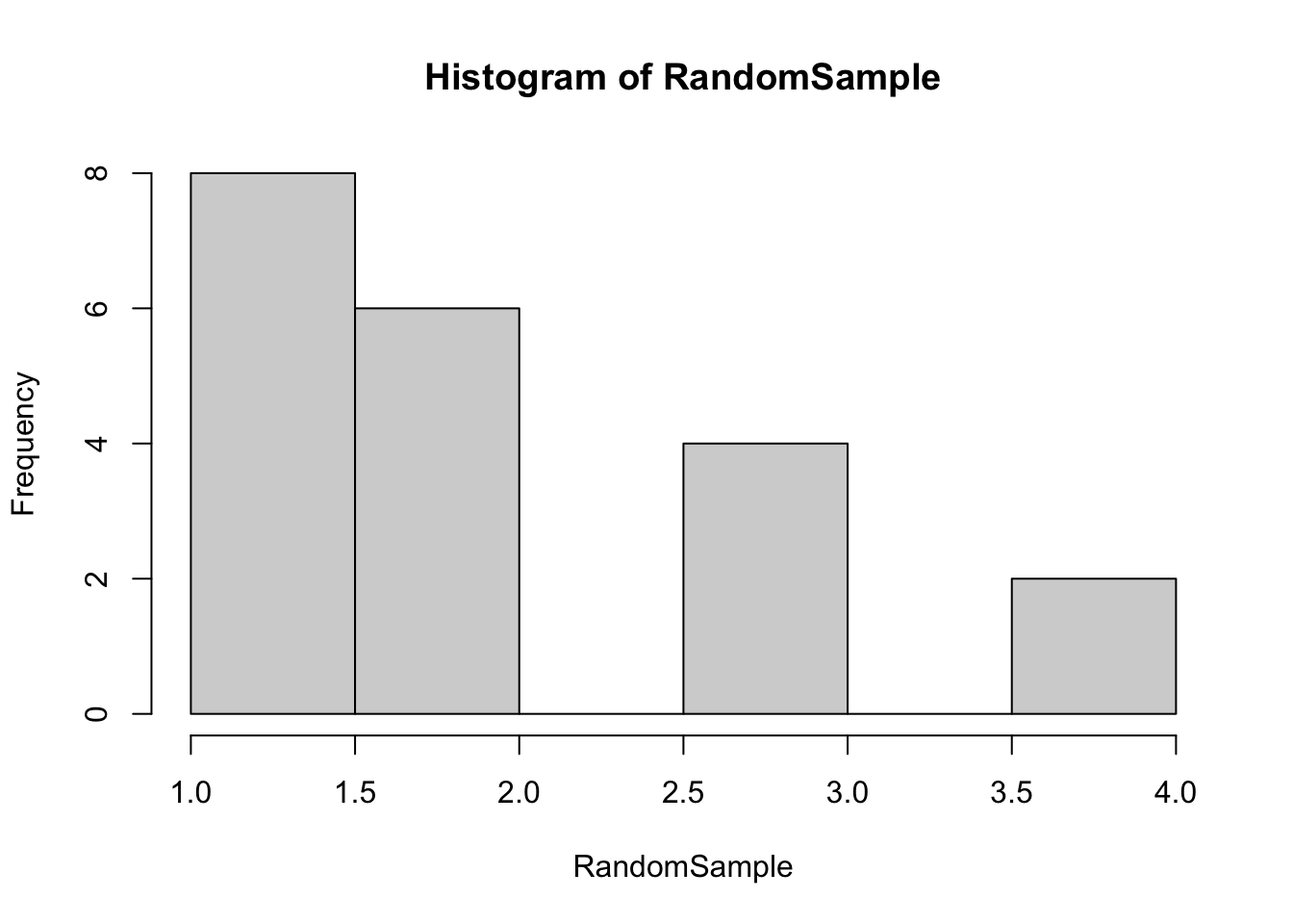
Repeat the example above, but change the mean of the Poisson distribution that you initially generate random numbers from.
This example considers creating a log-linear model for count data, i.e. Poisson regression. In the lectures, estimates of the parameters were just stated; now we will use R to obtain these. We will see the full details of the Surgery example and investigate whether Number of Surgery Visits is related to Location via a log-linear model. We assume a Poisson distributed dependent variable and independence.
library(foreign)
Surgery<-read.spss(file.choose(), to.data.frame = T)head(Surgery) Patient Location SurgeryVisits
1 1 0 1
2 2 0 2
3 3 1 5
4 4 1 6
5 5 1 5
6 6 0 1SurgeryPoissonReg<-glm(SurgeryVisits~factor(Location), data=Surgery, family="poisson")
summary(SurgeryPoissonReg)
Call:
glm(formula = SurgeryVisits ~ factor(Location), family = "poisson",
    data = Surgery)

Deviance Residuals:
    Min       1Q   Median       3Q      Max
-1.4138  -0.3379  -0.2238   0.1303   2.0000

Coefficients:
                  Estimate Std. Error z value Pr(>|z|)
(Intercept)         0.8473     0.2673   3.170  0.00152 **
factor(Location)1   0.7033     0.3190   2.205  0.02745 *
---
Signif. codes:  0 '***' 0.001 '**' 0.01 '*' 0.05 '.' 0.1 ' ' 1

(Dispersion parameter for poisson family taken to be 1)

    Null deviance: 14.1586  on 12  degrees of freedom
Residual deviance:  8.9034  on 11  degrees of freedom
AIC: 52.038

Number of Fisher Scoring iterations: 5anova(SurgeryPoissonReg, test="Chisq")Analysis of Deviance Table
Model: poisson, link: log
Response: SurgeryVisits
Terms added sequentially (first to last)
Df Deviance Resid. Df Resid. Dev Pr(>Chi)
NULL 12 14.1586
factor(Location) 1 5.2551 11 8.9034 0.02188 *
---
Signif. codes: 0 '***' 0.001 '**' 0.01 '*' 0.05 '.' 0.1 ' ' 1install.packages("lmtest")library(lmtest)
help("waldtest")
waldtest(SurgeryPoissonReg, test="Chisq")Wald test
Model 1: SurgeryVisits ~ factor(Location)
Model 2: SurgeryVisits ~ 1
Res.Df Df Chisq Pr(>Chisq)
1 11
2 12 -1 4.8621 0.02745 *
---
Signif. codes: 0 '***' 0.001 '**' 0.01 '*' 0.05 '.' 0.1 ' ' 1The Wald Chi-Square statistic is significant for Location (p-value of \(0.027<0.05\)) indicating the significance of the Location variable.
Further, from the earlier output, note that \(\hat{b}_0=0.847\); and \(\hat{b}_1=0.703\), i.e. we have the model, \[ \ln \hat{\lambda}_i=0.847+0.703x_{i1}, \text{ or } \hat{\lambda}_i=e^{0.847+0.703x_{i1}}=e^{0.847}(e^{0.703})^{x_{i1}}. \]
The Poisson Log-linear (PCP Defaults) dataset contains the number of defaults on personal contract plans (PCPs) for a certain car dealership according to their customers’ salary band. The Salary variable has 3 categories, 0, 1 and 2. Create a Poisson log-linear model for these data. You may assume independence and that the dependent variable is Poisson distributed. Make sure you analyse the output.
Hint: In this question the categorical variable (Salary) has more than 2 categories - this makes interpreting the model more complicated. The notes on dummy variables in the lecture notes should help you, along with Example 3 on the R examples class sheet.