help("pchisq")
pchisq(1.5,4)
[1] 0.1733585Please note that there is a file on Canvas called Getting started with R which may be of some use. This provides details of setting up R and Rstudio on your own computer as well as providing an overview of inputting and importing various data files into R. This should mainly serve as a reminder.
Recall that we can clear the environment using rm(list=ls()) It is advisable to do this before attempting new questions if confusion may arise with variable names etc.
In this example we will calculate various probabilities and critical values of chi-square distributions.
help("pchisq")
pchisq(1.5,4)[1] 0.1733585pchisq(0.25,4, lower.tail=F)[1] 0.992809qchisq(0.05,9, lower.tail = F)[1] 16.91898qchisq(0.01,12, lower.tail = F)[1] 26.21697a Let \(Y\sim\chi_7^2\), calculate \(P(0.5\leq Y<5.2)\). b Calculate the critical values \(\chi_{0.05,5}^2\) and \(\chi_{0.005,5}^2\).
pchisq(5.2,7)-pchisq(0.5,7)[1] 0.3638756qchisq(0.05,5, lower.tail = F)[1] 11.0705qchisq(0.005,5, lower.tail = F)[1] 16.7496In this example, we will perform the exam classification example, Example 3.1 in the lecture notes, in R. Recall that in this example we want to perform a chi-square goodness-of-fit test on the exams classification dataset below:
| A | B | C | D | E | |
|---|---|---|---|---|---|
| Observed (\(y_i\)) | 32 | 48 | 71 | 30 | 19 |
| Expected (\(\tilde{y}_i\)) | 20 | 40 | 80 | 40 | 20 |
Note: clearly the categories are independent and the expected frequencies are all \(\geq5\), hence satisfying the assumptions for categorical variables.
We first input the variables as below:
Class<-c("A", "B", "C", "D", "E")
Observed<-c(32,48,71,30,19)
Expected<-c(20,40,80,40,20)prop<-Expected/200
prop[1] 0.1 0.2 0.4 0.2 0.1ExamClass<-data.frame(Class,Observed,Expected,prop)chisq.test(Observed,p=prop)
    Chi-squared test for given probabilities

data:  Observed
X-squared = 12.363, df = 4, p-value = 0.01485
You should obtain a p-value of \(0.01485<0.05\) as per the above output, therefore we reject the null hypothesis that the exam results follow the expected distribution. Note that this does not highlight where the discrepancies lie.
We next produce side-by-side bar charts to visualise the observed versus expected frequencies. We must first create a matrix containing the observed and expected frequencies, see below.
ExamClassMatrix<-matrix(c(32,20,48,40,71,80,30,40,19,20), nrow=2,
              dimnames = list(c("Observed","Expected"), c("A","B","C","D","E")))
ExamClassMatrix
A B C D E
Observed 32 48 71 30 19
Expected 20 40 80 40 20barplot(ExamClassMatrix,
beside=TRUE,
ylim=c(0, 100),legend=T, col=c("yellow","blue"),
xlab="Exam Classifications",
ylab="Frequency")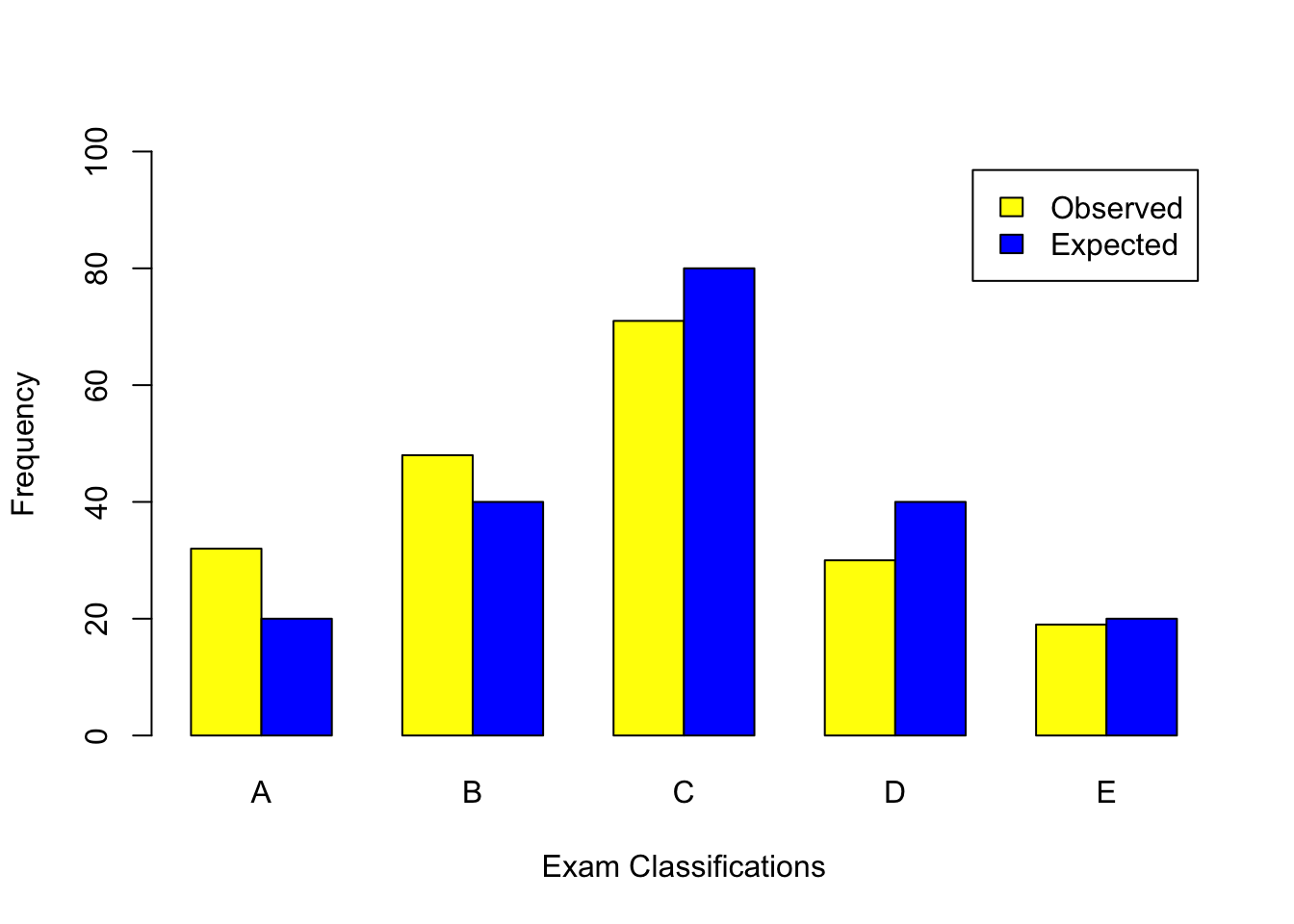
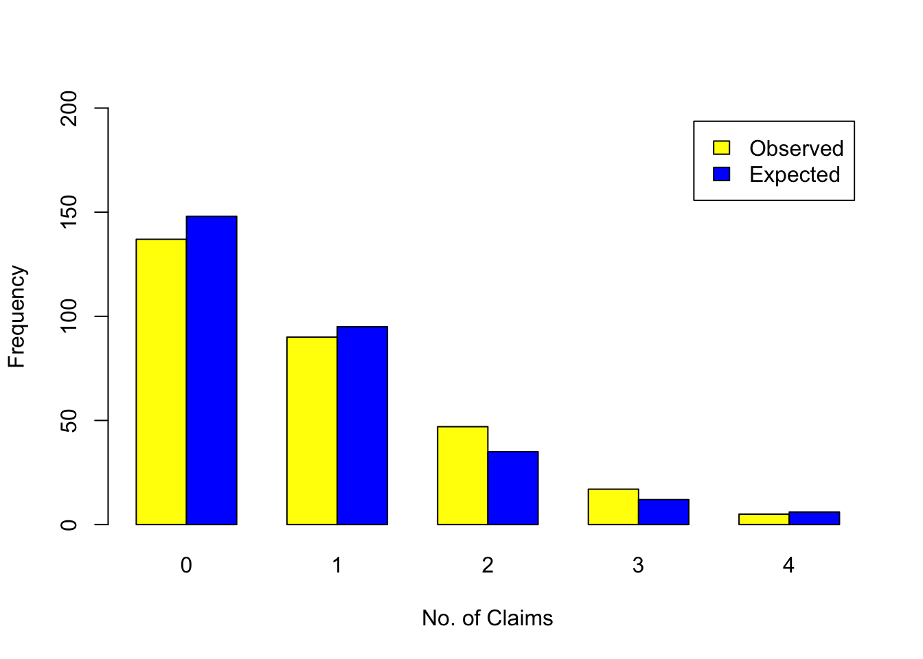
The table below contains the observed and expected number of car insurance claims per policy holder in a given year.
| Claims: | 0 | 1 | 2 | 3 | 4 | |
|---|---|---|---|---|---|---|
| Observed | 137 | 90 | 47 | 17 | 5 | |
| Expected | 148 | 95 | 35 | 12 | 6 |
Checking the assumptions for categorical variables, perform a \(\chi^2\) goodness-of-fit test on this dataset.
Claims<-c(0,1,2,3,4)
Observed2<-c(137,90,47,17,5)
Expected2<-c(148,95,35,12,6)prop2<-Expected2/296ClaimsData<-data.frame(Claims,Observed2,Expected2, prop2)
ClaimsData Claims Observed2 Expected2 prop2
1 0 137 148 0.50000000
2 1 90 95 0.32094595
3 2 47 35 0.11824324
4 3 17 12 0.04054054
5 4 5 6 0.02027027chisq.test(Observed2,p=prop2)
    Chi-squared test for given probabilities

data:  Observed2
X-squared = 7.445, df = 4, p-value = 0.1142
The p-value is 0.1142 therefore we do not reject the null hypothesis and conclude that the data is as expected.
Finally, we produce bar charts of the observed and expected frequencies for each claims number.
ClaimsMatrix<-matrix(c(137,148,90,95,47,35,17,12,5,6), nrow=2, dimnames = list(c("Observed","Expected"), c("0","1","2","3","4")))
ClaimsMatrix
0 1 2 3 4
Observed 137 90 47 17 5
Expected 148 95 35 12 6barplot(ClaimsMatrix,
beside=TRUE,
ylim=c(0, 200),legend=T, col=c("yellow","blue"),
xlab="No. of Claims",
ylab="Frequency")