Lab 2 - with solutions

Please note that there is a file on Canvas called Getting started with R which may be of some use. This provides details of setting up R and Rstudio on your own computer as well as providing an overview of inputting and importing various data files into R. This should mainly serve as a reminder.

Recall that we can clear the environment using rm(list=ls()) It is advisable to do this before attempting new questions if confusion may arise with variable names etc.

Example 1

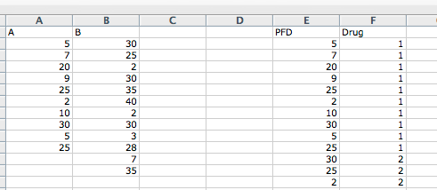
In this example we will elaborate on one of the lecture examples where we investigated the effectiveness of two different asthma drugs. The data is provided in the Asthma Drugs dataset, and the readings are peak flow meter differences for the two drugs. The dataset must first be adapted into an R friendly form, i.e. create a new column with all the peak flow measurements in one column, which I have called PFD, with an associated grouping variable, which I have called Drug. Remember to save your file as a csv file. Below is a snippet of my revised dataset:

Next, follow the step-by-step guide below,

Firstly, we input the dataset into R, check it using the “head” command (recall this provides the first 6 entries) and attach it.

Asthma<-read.csv(file.choose(), header=T)

Asthma<-read.csv("Asthma Drugs Revised.csv", header=T)
head(Asthma)

   A  B  X X.1 PFD Drug
1  5 30 NA  NA   5    1
2  7 25 NA  NA   7    1
3 20  2 NA  NA  20    1
4  9 30 NA  NA   9    1
5 25 35 NA  NA  25    1
6  2 40 NA  NA   2    1

attach(Asthma)

If the two samples are normally distributed then this would be the situation of an independent samples t-test (seen in MA-192). Therefore, we will first check the normality of drugs A and B. To do this, use the following code

shapiro.test(A)


    Shapiro-Wilk normality test

data:  A
W = 0.87786, p-value = 0.1233

shapiro.test(B)


    Shapiro-Wilk normality test

data:  B
W = 0.82685, p-value = 0.01923

and

install.packages("nortest")

library(nortest)
lillie.test(A)


    Lilliefors (Kolmogorov-Smirnov) normality test

data:  A
D = 0.24576, p-value = 0.08832

lillie.test(B)


    Lilliefors (Kolmogorov-Smirnov) normality test

data:  B
D = 0.24234, p-value = 0.04996

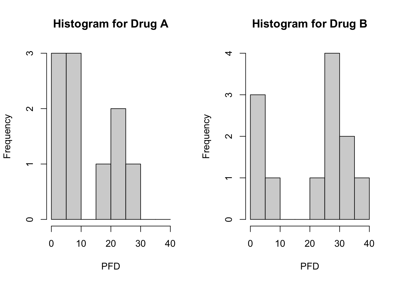
Clearly the data are not normally distributed, therefore we proceed with the non-parametric equivalent test, the Mann-Whitney U-test. Before doing this, we investigate the shape of the distributions of the data. We will do this by creating histograms of the data. We create a factor for Drug and create side-by-side histograms for an easier comparison, noting the choice of “breaks” to provide better presentation, see the code below:

Drug<-factor(Drug,c(1,2),labels=c('Drug A','Drug B'))
par(mfrow=c(1,2)) 
hist(PFD[Drug=='Drug A'], xlab='PFD', main='Histogram for Drug A', breaks=seq(from=0,to=40,by=5)) 
hist(PFD[Drug=='Drug B'], xlab='PFD', main='Histogram for Drug B', breaks=seq(from=0,to=40,by=5))

The histograms produced should show that both drugs have similar shaped distributions. Recall from the lectures that this allows us to effectively compare medians using the Mann-Whitney U-test. Without this, we would be testing whether the two groups follow the same distribution.
To perform the Mann-Whitney U-test, use the code below (Please note that the default option for pairing is false, i.e. a Mann-Whitney U test and not a Wilcoxon Signed-Rank test):

wilcox.test(PFD~Drug)

You will have obtain an error concerning ties when you use this approach. For cases where we have ties in the data we have to use the option ``exact=F”, see below:

wilcox.test(PFD~Drug, exact=F)


    Wilcoxon rank sum test with continuity correction

data:  PFD by Drug
W = 39, p-value = 0.1739
alternative hypothesis: true location shift is not equal to 0

Note that we may use the original data, i.e. side-by-side columns, but we have to adapt the code slightly to:

wilcox.test(A,B, exact=F)


    Wilcoxon rank sum test with continuity correction

data:  A and B
W = 39, p-value = 0.1739
alternative hypothesis: true location shift is not equal to 0

In both approaches check that you obtain a p-value of \(0.1739>0.05\), therefore we do not reject \(H_0\) and conclude that there is no difference between the medians of the two asthma drugs.
Please note that there is also the wilcox_test command within the “coin” package that can deal with ties, see

install.packages("coin")

library(coin)
wilcox_test(PFD~Drug)


    Asymptotic Wilcoxon-Mann-Whitney Test

data:  PFD by Drug (Drug A, Drug B)
Z = -1.393, p-value = 0.1636
alternative hypothesis: true mu is not equal to 0

We obtain the same conclusion with this technique.

Exercise 1

The Reaction Times dataset contains the results of a trial measuring reaction times of 2 different groups of people, where one group is given water before the trial and the other group is given a new drink designed to reduce reaction times. Perform an appropriate statistical test to determine whether there is any difference in reaction times. Calculate the effect size.

Hint: Note that in order to obtain a \(Z\) value to calculate the effect size, the wilcox_test() command from the “coin” package will need to be used. Also remember how to import an SPSS file: either using the foreign package or use the Import Dataset command under Environment.

Solutions

Importing the data:

library(foreign)
ReactionData<- read.spss(file.choose(), to.data.frame=T)

We first investigate the normality of the groups to determine the appropriate test.

shapiro.test(ReactionData$NewDrink)


    Shapiro-Wilk normality test

data:  ReactionData$NewDrink
W = 0.86864, p-value = 0.03223

shapiro.test(ReactionData$Water)


    Shapiro-Wilk normality test

data:  ReactionData$Water
W = 0.83015, p-value = 0.009204

library(nortest)
lillie.test(ReactionData$NewDrink)


    Lilliefors (Kolmogorov-Smirnov) normality test

data:  ReactionData$NewDrink
D = 0.22467, p-value = 0.04019

lillie.test(ReactionData$Water)


    Lilliefors (Kolmogorov-Smirnov) normality test

data:  ReactionData$Water
D = 0.23322, p-value = 0.02749

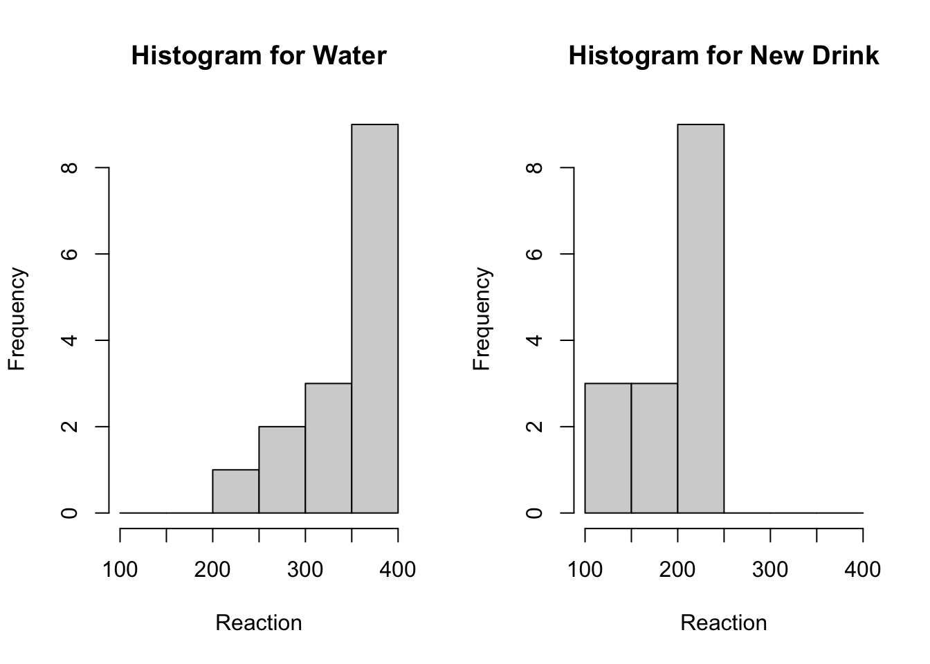
The output of the test indicate the groups are not normally distributed, hence we use a Mann-Whitney U test. In order to determine the correct hypotheses we investigate the shape of the groups.

DrinkType<-factor(ReactionData$Drink,c(1,2),labels=c('Water','New Drink'))

par(mfrow=c(1,2)) 
hist(ReactionData$ReactionTime[ReactionData$Drink=='Water'], xlab='Reaction', main='Histogram for Water', breaks=seq(from=100,to=400, by=50)) 
hist(ReactionData$ReactionTime[ReactionData$Drink=='New Drink'], xlab='Reaction', main='Histogram for New Drink', breaks=seq(from=100,to=400, by=50))

The groups seem to be of a similar shape, hence we compare group medians in the Mann-Whitney U test.

wilcox.test(ReactionData$ReactionTime~ReactionData$Drink)

Warning in wilcox.test.default(x = DATA[[1L]], y = DATA[[2L]], ...): cannot
compute exact p-value with ties


    Wilcoxon rank sum test with continuity correction

data:  ReactionData$ReactionTime by ReactionData$Drink
W = 1, p-value = 4.012e-06
alternative hypothesis: true location shift is not equal to 0

Since there are ties in the dataset we use:

wilcox.test(ReactionData$ReactionTime~ReactionData$Drink, exact=F)


    Wilcoxon rank sum test with continuity correction

data:  ReactionData$ReactionTime by ReactionData$Drink
W = 1, p-value = 4.012e-06
alternative hypothesis: true location shift is not equal to 0

Or we can use the coin package and use the code below (which provides a Z value that will need to be used to calculate the effect size)

library(coin)
wilcox_test(ReactionData$ReactionTime~ReactionData$Drink)


    Asymptotic Wilcoxon-Mann-Whitney Test

data:  ReactionData$ReactionTime by ReactionData$Drink (New Drink, Water)
Z = -4.6315, p-value = 3.63e-06
alternative hypothesis: true mu is not equal to 0

As we have a significant result it is good practice to compare medians.

tapply(ReactionData$ReactionTime,ReactionData$Drink,median)

New Drink     Water 
      220       370

The effect size is given by, \[ r=\frac{Z}{\sqrt{n}}, \] where \(n=n_1+n_2\).
In this exercise, we have \[ r=\frac{-4.632}{\sqrt{30}}=0.85, \] i.e. a large effect size.

Example 2

In this example we will perform Example 2.9 in R. Using the Public Awareness dataset, we investigate whether there is any difference between a certain video (Video A) and a method using props (Demo D) in informing the public about a certain medical condition. The same participants evaluate each method. Please follow the steps below:

Firstly use the “Import Dataset” command in the “Environment” to import the dataset.
We could be mistaken to think that this is a situation where we use a paired t-test. Perform a test of normality on the differences to check one of the main conditions of this test using,

shapiro.test(Public_Awareness$Difference)


    Shapiro-Wilk normality test

data:  Public_Awareness$Difference
W = 0.95299, p-value = 0.4147

install.packages("nortest")

library(nortest)
lillie.test(Public_Awareness$Difference)


    Lilliefors (Kolmogorov-Smirnov) normality test

data:  Public_Awareness$Difference
D = 0.15672, p-value = 0.2223

Note that we do not have evidence to reject the normality of the data. However, if we look carefully at the dataset, we see that we are dealing with ordinal data and therefore the Wilcoxon Signed-Rank test is an option (the assumption of continuous data of the paired t-test is not met since there are only 4 ordered categories - recall that 7 or more are required to be classed as continuous).
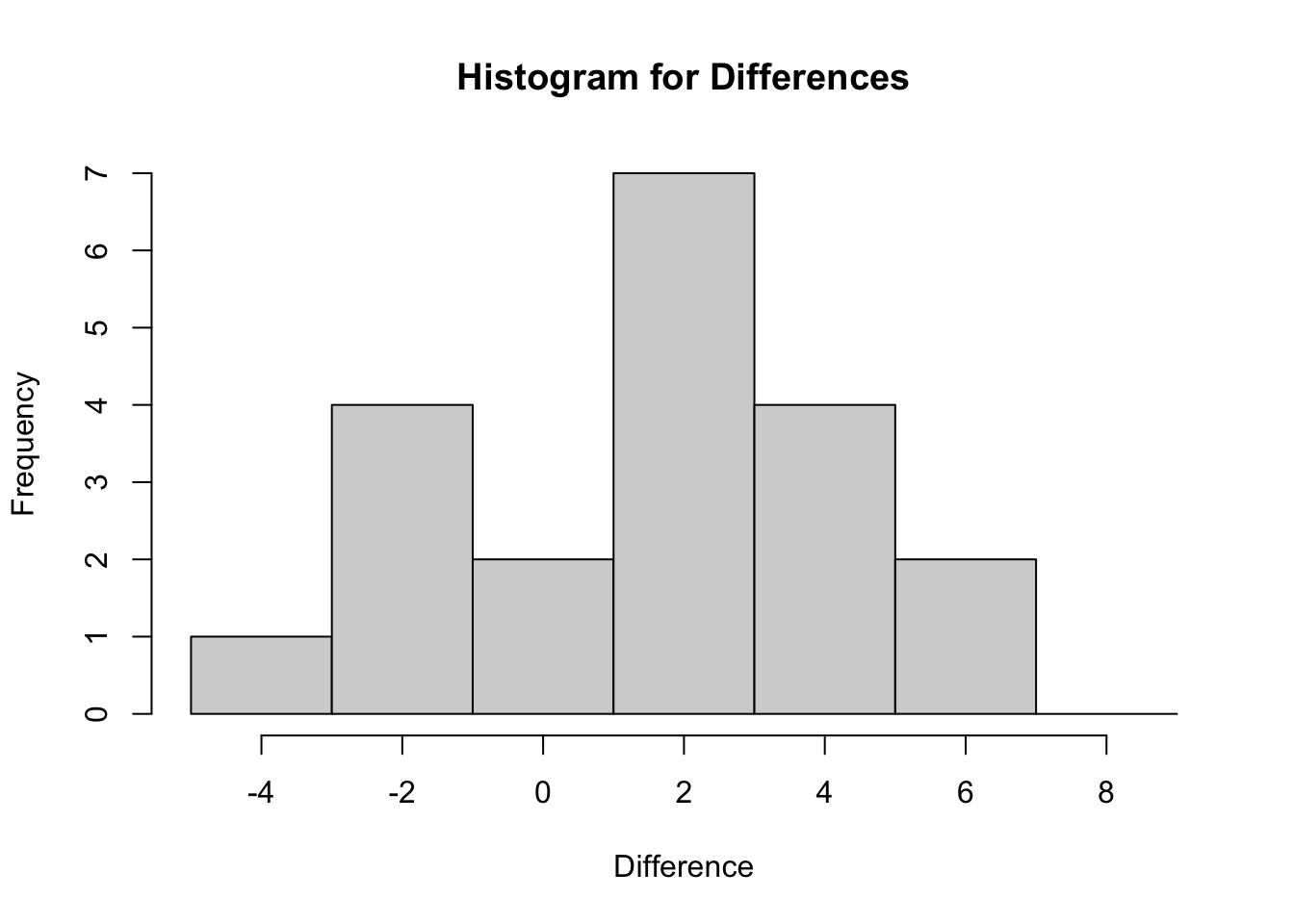
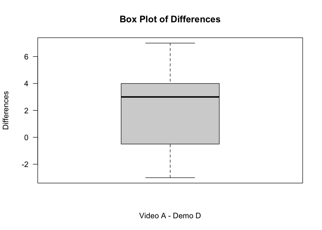
We next investigate the shape of the differences using a histogram and boxplot in order to determine the correct hypotheses, see

hist(Public_Awareness$Difference, xlab='Difference', main='Histogram for Differences', breaks=seq(from=-5,to=10, by=2))

boxplot(Public_Awareness$Difference, main="Box Plot of Differences", ylab="Differences", xlab="Video A - Demo D", las=1)

From your output you should be able to see that the differences do appear to be symmetric.
Now we proceed to the Wilcoxon Signed-Rank test.

wilcox.test(Public_Awareness$TotalAGen, Public_Awareness$TotalDDEMO, paired=TRUE, exact=F)


    Wilcoxon signed rank test with continuity correction

data:  Public_Awareness$TotalAGen and Public_Awareness$TotalDDEMO
V = 167.5, p-value = 0.003558
alternative hypothesis: true location shift is not equal to 0

The test statistic is significant, therefore we conclude that median difference is significantly different to 0.
The medians can be calculated using

median(Public_Awareness$TotalAGen)

[1] 24

median(Public_Awareness$TotalDDEMO)

[1] 22

As the median of Video A is 24 and that of Demo D is 22, we conclude that Video A seems to be more effective.
The coin package has an alternative function for this procedure, however the data must be presented differently, i.e. one column containing the data and a grouping variable. I have created a new file called Public Awareness Revised to do this. Import this dataset and use the relevant code below:

wilcoxsign_test(Public_Awareness_Revised$Effectiveness~Public_Awareness_Revised$Method)


    Asymptotic Wilcoxon-Pratt Signed-Rank Test

data:  y by x (pos, neg) 
     stratified by block
Z = 5.5779, p-value = 2.434e-08
alternative hypothesis: true mu is not equal to 0

Exercise 2

The Reorganisation Salaries dataset contains the salaries of individual employees before and after a reorganisation. Investigate whether there is any statistically significant difference in the salaries before and after the reorganisation, justifying fully the procedure used.

Hint: The differences are not provided in the dataset, therefore you must create a new dataset which includes a new column containing the differences. Either do this in Excel before importing the data or use the following code in R:

Salaries.new <- transform(Salaries, Differences = Before - After)
Salaries.new

Solutions

Importing the data:

Salaries<-read.csv(file.choose(), header=T)
head(Salaries)

  Before After
1  20000 25000
2  36000 45000
3  26000 19000
4  26000 14000
5  73000 89000
6  34000 23000

The differences are not provided in the dataset, therefore we must create a new dataset which includes a new column containing the differences.

Salaries.new <- transform(Salaries, Differences = Before - After)
Salaries.new

   Before  After Differences
1   20000  25000       -5000
2   36000  45000       -9000
3   26000  19000        7000
4   26000  14000       12000
5   73000  89000      -16000
6   34000  23000       11000
7  149000 147000        2000
8   66000  50000       16000
9   23000  24000       -1000
10  20000  30000      -10000
11  80000  68000       12000
12  85000 159000      -74000

We next test the normality of the differnecs to determine which technique is suitable.

shapiro.test(Salaries.new$Differences)


    Shapiro-Wilk normality test

data:  Salaries.new$Differences
W = 0.72446, p-value = 0.001465

library(nortest)
lillie.test(Salaries.new$Differences)


    Lilliefors (Kolmogorov-Smirnov) normality test

data:  Salaries.new$Differences
D = 0.24453, p-value = 0.04588

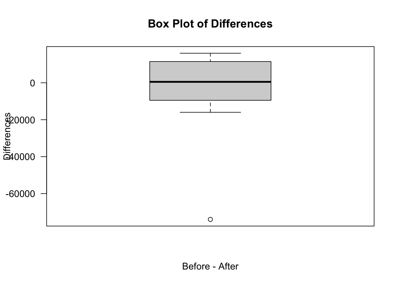
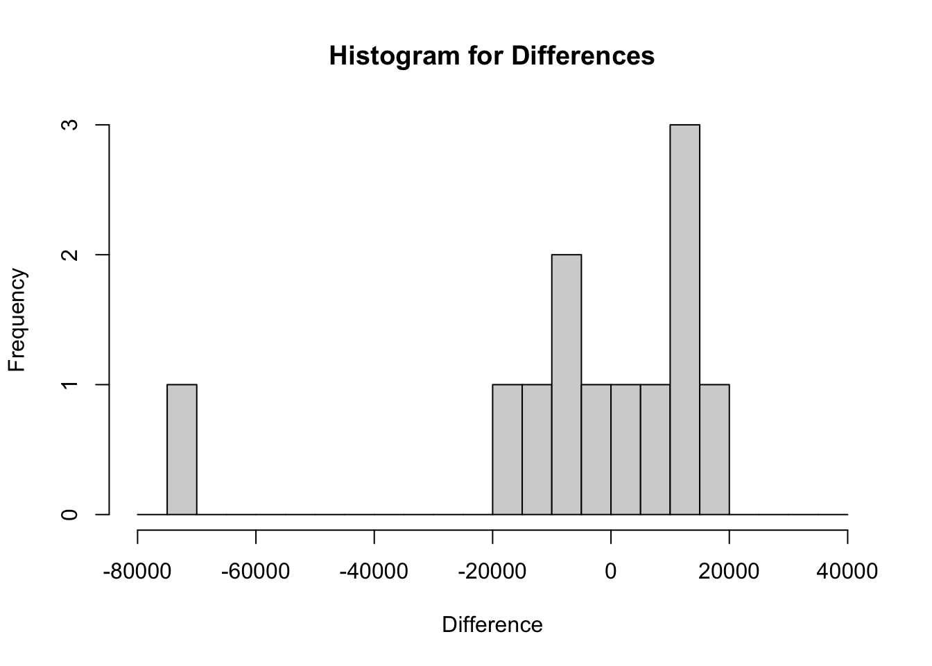
Since the differneces do not appear to be normally distributed we procedd with the Wilcoxon Signed-Rank test, however we first determine whether the differences are symmetric.

boxplot(Salaries.new$Differences, main="Box Plot of Differences", ylab="Differences", xlab="Before - After", las=1)

hist(Salaries.new$Differences, xlab='Difference', main='Histogram for Differences', breaks=seq(from=-80000,to=40000, by=5000))

The differences appear to be symmetric, hence we continue with our test.

wilcox.test(Salaries.new$Before, Salaries.new$After, paired=TRUE)

As there is a warning about ties, we use:

wilcox.test(Salaries.new$Before, Salaries.new$After, paired=TRUE, exact=F)


    Wilcoxon signed rank test with continuity correction

data:  Salaries.new$Before and Salaries.new$After
V = 40.5, p-value = 0.9374
alternative hypothesis: true location shift is not equal to 0

Now we see that the result is not significant indicating that there does not appear to be any difference between the median salary before and after the reorganisation.